Here are some solutions for the exercises from Week 5.
If you have questions, comments, or find something that looks like a mistake, feel free to email me at oskar.henriksson@math.ku.dk!
Remark: The HomotopyContinuation.jl package is developed by different people than the group of people who develop OSCAR, so the commands, output and underlying data types are a bit different from what you're used to from OSCAR. This will take a while to get used to!
Recommendation: To avoid confusion with the data types, we recommend that you always run HomotopyContinuation.jl code and OSCAR code in separate Jupyter notebooks, and that you manually copy and paste data between them.
If you haven't installed HomotopyContinuation.jl yet, you can do this with the package manager. The surest way to get the latest version is to install directly from the github repository.
#using Pkg
#Pkg.add(url="https://github.com/JuliaHomotopyContinuation/HomotopyContinuation.jl")
You can check that you have the latest version (v2.6.4) with the help of the Pkg.status command.
using Pkg
Pkg.status("HomotopyContinuation")
Status `~/.julia/environments/v1.8/Project.toml`
  [f213a82b] HomotopyContinuation v2.6.4 `https://github.com/JuliaHomotopyContinuation/HomotopyContinuation.jl#main`
using HomotopyContinuation
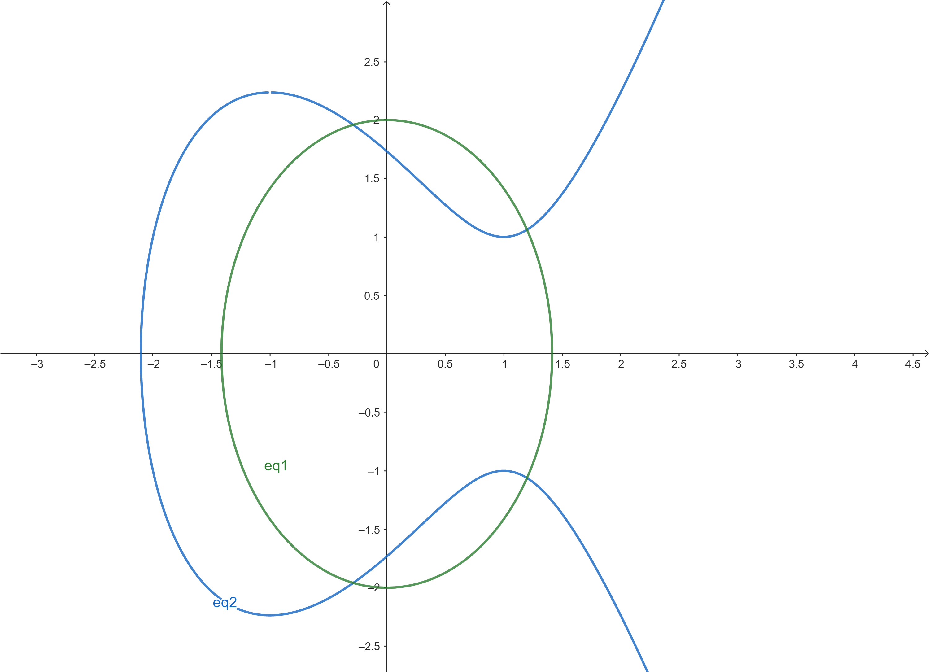
In this problem, we find all the complex intersection points between an ellipse and an elliptic curve, given by the system
$$\begin{cases}2x^2+y^2-4=0\\x^3-3x-y^2+3=0\,.\end{cases}$$A routine check in OSCAR (see code from Week 4) reveals that the ideal
is radical, and $\dim_{\mathbb{C}}(C[x,y]/I)=6$, so we know that $$\#\mathbb{V}(I)=6\,.$$
This agrees completely with the Bézout bound, which is $2\cdot 3=6$.
The total degree start system looks as follows (note that we abuse notation a bit by abbreviating the variable vector $(x,y)$ by $x$ in the left-hand side):
$$G(x)=\begin{bmatrix}x^2-1\\y^3-1\end{bmatrix}.$$The straight-line homotopy (with the $\gamma$-trick) is $$H(t,x)=(t-1)\gamma G(x)+tF(x)=\left[ \begin {array}{c} \left( 1-t \right) \gamma\, \left( {x}^{2}- 1 \right) +t \left( 2\,{x}^{2}+{y}^{2}-4 \right) \\ \left( 1-t \right) \gamma\, \left( {y}^{3}-1 \right) +t \left( {x}^{3 }-{y}^{2}-3\,x+3 \right) \end {array} \right].$$
To write down the Davidenko differential equation, we need to differentiate $H$ with respect to both the variables and the parameter $t$.
The Jacobian with respect to the variables is $$\frac{\partial H}{\partial x}=\left[ \begin {array}{cc} 2\, \left( 1-t \right) \gamma\,x+4\,tx&2\,t y\\ t \left( 3\,{x}^{2}-3 \right) &3\, \left( 1-t \right) \gamma\,{y}^{2}-2\,ty\end {array} \right].$$
The derivative with respect to $t$ is $$ \frac{\partial H}{\partial t} = \left[ \begin {array}{c} -\gamma\, \left( {x}^{2}-1 \right) +2\,{x}^{ 2}+{y}^{2}-4\\ -\gamma\, \left( {y}^{3}-1 \right) +{ x}^{3}-{y}^{2}-3\,x+3\end {array} \right].$$
All in all, we obtain $$\frac{dx}{dt}=-\left(\frac{\partial H}{\partial x}\right)^{-1}\frac{\partial H}{\partial t}=-\left[ \begin {array}{cc} 2\, \left( 1-t \right) \gamma\,x+4\,tx&2\,t y\\ t \left( 3\,{x}^{2}-3 \right) &3\, \left( 1-t \right) \gamma\,{y}^{2}-2\,ty\end {array} \right]^{-1} \left[ \begin {array}{c} -\gamma\, \left( {x}^{2}-1 \right) +2\,{x}^{ 2}+{y}^{2}-4\\ -\gamma\, \left( {y}^{3}-1 \right) +{ x}^{3}-{y}^{2}-3\,x+3\end {array} \right]\,.$$
The first step is to define the variables, and create the system.
@var x y;
F = System( [2*x^2+y^2-4, x^3-3*x-y^2+3] )
System of length 2
 2 variables: x, y

 -4 + 2*x^2 + y^2
 3 - 3*x + x^3 - y^2
To solve the system with homotopy continuation, we use the solve command.
res = solve(F, start_system = :total_degree)
Tracking 6 paths... 100%|███████████████████████████████| Time: 0:00:17
  # paths tracked:                  6
  # non-singular solutions (real):  6 (4)
  # singular endpoints (real):      0 (0)
  # total solutions (real):         6 (4)
Result with 6 solutions
=======================
• 6 paths tracked
• 6 non-singular solutions (4 real)
• random_seed: 0xdb2529d7
• start_system: :total_degree
The output from solve is an abstract data type called "result" that contains lots of additional information, other than just the solutions. You can access the actual solutions by applying the solutions command.
sol = solutions(res)
6-element Vector{Vector{ComplexF64}}:
 [1.198691243515997 + 0.0im, 1.0612627410006181 - 2.2420775429197073e-44im]
 [-0.28646206503160054 - 6.305843089461677e-45im, 1.9585400099552885 + 0.0im]
 [-2.912229178484397 + 0.0im, 1.1479437019748901e-41 - 3.6002996508668286im]
 [-2.9122291784843966 + 1.1754943508222875e-38im, 2.350988701644575e-38 + 3.600299650866828im]
 [1.198691243515997 + 2.9846536251347144e-40im, -1.061262741000618 - 3.6734198463196485e-40im]
 [-0.2864620650316005 - 1.5694542800437951e-43im, -1.9585400099552888 + 0.0im]
The command for doing certification is certify.
cert_res = certify(F, sol)
CertificationResult
===================
• 6 solution candidates given
• 6 certified solution intervals (4 real, 2 complex)
• 6 distinct certified solution intervals (4 real, 2 complex)
We can obtain the data from the certification result with the command certificates, but this easily gets a bit overwhelming, so it's usually easier to loop through the certificates and ask for specific information.
#certificates(cert_res)
The following script loops through all the six boxes (so-called certified solution intervals) that the program has found, and prints the box together with information about whether the program was able to verify that the corresponding solution is real.
true means that the solution is verifiably real, whereas false just means that it couldn't verify realness. To be sure that the solution is nonreal, you have to look at the box yourself and convince yourself that it doesn't contain any real points.
for c in certificates(cert_res)
    display(c.index) #the index number of the solution
    display( certified_solution_interval(c) ) #the box that encloses the true solution
    display( is_real(c) ) #is the true solution verifiably real?
    print("\n") #line break for readability
end
1
2×1 Arblib.AcbMatrix:
 [1.198691243516 +/- 5.06e-13] + [+/- 5.03e-13]im
  [1.06126274100 +/- 1.35e-12] + [+/- 7.31e-13]im
true
2
2×1 Arblib.AcbMatrix:
 [-0.286462065032 +/- 9.25e-13] + [+/- 5.25e-13]im
  [1.958540009955 +/- 6.21e-13] + [+/- 3.32e-13]im
true
3
2×1 Arblib.AcbMatrix:
 [-2.91222917848 +/- 6.63e-12] + [+/- 2.24e-12]im
 [+/- 5.00e-12] + [-3.60029965087 +/- 8.18e-12]im
false
4
2×1 Arblib.AcbMatrix:
 [-2.91222917848 +/- 6.63e-12] + [+/- 2.24e-12]im
  [+/- 5.00e-12] + [3.60029965087 +/- 8.18e-12]im
false
5
2×1 Arblib.AcbMatrix:
 [1.198691243516 +/- 5.06e-13] + [+/- 5.03e-13]im
 [-1.06126274100 +/- 1.35e-12] + [+/- 7.31e-13]im
true
6
2×1 Arblib.AcbMatrix:
 [-0.286462065032 +/- 9.25e-13] + [+/- 5.25e-13]im
 [-1.958540009955 +/- 6.21e-13] + [+/- 3.32e-13]im
true
Conclusions:
We saw in part (a) of this problem that there should be 6 solutions of this system.
Since certification shows that we have found 6 distinct solutions, we know we haven't missed any solutions.
Among these 6 solutions, we saw in part (d) that preciely one is positive.
Hence, the above constitutes a proof that the system has a unique positive real solution!
@var x y z
F = System([x^2+y^2+z^2-1,x^2+y^2+z^2-2*x,2*x-3*y-z])
System of length 3
 3 variables: x, y, z

 -1 + x^2 + y^2 + z^2
 -2*x + x^2 + y^2 + z^2
 2*x - 3*y - z
sol1 = [0.5000000000, 0.55495098, -0.664852927]
3-element Vector{Float64}:
  0.5
  0.55495098
 -0.664852927
sol2 = [0.5000000000, 0.045049024, 0.86485293]
3-element Vector{Float64}:
 0.5
 0.045049024
 0.86485293
cert_res = certify(F, [sol1,sol2])
CertificationResult
===================
• 2 solution candidates given
• 2 certified solution intervals (2 real, 0 complex)
• 2 distinct certified solution intervals (2 real, 0 complex)
for c in certificates(cert_res)
    display(certified_solution_interval(c))
end
3×1 Arblib.AcbMatrix:
  [0.500000000000 +/- 3.70e-13] + [+/- 3.70e-13]im
  [0.554950975680 +/- 6.52e-13] + [+/- 2.91e-13]im
 [-0.664852927039 +/- 3.95e-13] + [+/- 3.13e-13]im
3×1 Arblib.AcbMatrix:
 [0.500000000000 +/- 3.70e-13] + [+/- 3.70e-13]im
 [0.045049024320 +/- 6.81e-13] + [+/- 3.20e-13]im
 [0.864852927039 +/- 3.05e-13] + [+/- 2.23e-13]im
We see that the boxes obtained with certify are a lot more refined than the solution intervals that we obtained in Week 3!
(In particular, the approximations we started with don't belong to the new boxes!)
If we want to work with the refined solutions instead of the solutions we started with, we can access them in the following way:
for c in certificates(cert_res)
    display(c.solution)
end
3-element Vector{ComplexF64}:
                 0.5 + 0.0im
  0.5549509756796391 + 0.0im
 -0.6648529270389177 + 0.0im
3-element Vector{ComplexF64}:
                  0.5 + 0.0im
 0.045049024320360787 + 0.0im
   0.8648529270389177 + 0.0im
...or we can store them in a list for later use like this:
refined_sol = [c.solution for c in certificates(cert_res)]
2-element Vector{Vector{ComplexF64}}:
 [0.5 + 0.0im, 0.5549509756796391 + 0.0im, -0.6648529270389177 + 0.0im]
 [0.5 + 0.0im, 0.045049024320360787 + 0.0im, 0.8648529270389177 + 0.0im]
certify are virtually indistinguishable from the original solutions.
As explained in the problem text, we want to solve the following system:
$$\begin{cases}f(x_1,x_2)=0\\ \tfrac{df}{dx_1}(x_1,x_2)-\lambda(x_1-u_1)=0\\ \tfrac{df}{dx_2}(x_1,x_2)-\lambda(x_2-u_2)=0\,.\end{cases}$$You can either differentiate $f$ by hand, or use the command differentiate from the HomotopyContinuation.jl.
@var x[1:2] lambda;
u = [1,2]
2-element Vector{Int64}:
 1
 2
f = x[1]^2*x[2]^2-3*x[1]^2-3*x[2]^2+5
F = System([f,
        differentiate(f,x[1])-lambda*(x[1]-u[1]),
        differentiate(f,x[2])-lambda*(x[2]-u[2])])
System of length 3
 3 variables: lambda, x₁, x₂

 5 + x₂^2*x₁^2 - 3*x₁^2 - 3*x₂^2
 -6*x₁ + 2*x₂^2*x₁ - (-1 + x₁)*lambda
 -6*x₂ + 2*x₂*x₁^2 - (-2 + x₂)*lambda
res = solve(F,start_system = :total_degree)
Tracking 36 paths... 100%|██████████████████████████████| Time: 0:00:05
  # paths tracked:                  36
  # non-singular solutions (real):  12 (6)
  # singular endpoints (real):      0 (0)
  # total solutions (real):         12 (6)
Result with 12 solutions
========================
• 36 paths tracked
• 12 non-singular solutions (6 real)
• random_seed: 0x38304250
• start_system: :total_degree
sol = solutions(res)
12-element Vector{Vector{ComplexF64}}:
 [7.337456669889568 - 1.5407439555097887e-33im, 0.6974628316032541 + 4.81482486096809e-35im, 1.1868540198708355 + 0.0im]
 [-6.684913507776384 + 5.632365503258928im, 1.574816759003061 - 0.550283425679337im, 1.5702213850781328 + 0.5997392554527856im]
 [-6.684913507776384 - 5.632365503258928im, 1.574816759003061 + 0.5502834256793371im, 1.5702213850781326 - 0.5997392554527857im]
 [12.52659539322109 - 1.4693679385278594e-39im, 2.0594737601345003 + 0.0im, 2.4944107570298666 - 2.7550648847397363e-40im]
 [-2.300890888977063 + 2.828521937480216im, -1.4769430321350407 + 0.32319544893386803im, 1.2754681657127243 + 0.8488645234473869im]
 [-2.300890888977063 - 2.8285219374802164im, -1.4769430321350407 - 0.3231954489338682im, 1.2754681657127243 - 0.8488645234473868im]
 [6.180582548943949 + 1.232595164407831e-32im, -1.9641008231775792 - 3.851859888774472e-34im, 2.7683349808147066 + 1.5407439555097887e-33im]
 [-2.5791116761389627 + 1.4069820017154362im, 0.8002675218685461 + 0.91971767752603im, -1.4133261659627496 + 0.1674260779939675im]
 [-2.5791116761389627 - 1.4069820017154364im, 0.8002675218685461 - 0.91971767752603im, -1.4133261659627496 - 0.16742607799396744im]
 [3.6307861905992644 + 0.0im, 2.570315873979099 - 1.88079096131566e-37im, -2.0270918252578882 + 9.4039548065783e-38im]
 [-1.6232400471262118 - 4.203895392974451e-45im, -0.8541685916254985 + 4.203895392974451e-45im, -1.112741129782544 + 1.226136156284215e-45im]
 [2.4109847235904964 + 0.0im, -2.3052655483869082 + 0.0im, -2.1744935723311904 + 4.591774807899561e-41im]
The variables are ordered alphabetically by default, i.e. $\lambda,x_1,x_2$. We only care about $x_1$ and $x_2$ (so the second and third coordinate of all the solution vectors), so let's extract these!
for s in solutions(res)
    display(s[2:3])
end
2-element Vector{ComplexF64}:
 0.6974628316032541 + 4.81482486096809e-35im
 1.1868540198708355 + 0.0im
2-element Vector{ComplexF64}:
  1.574816759003061 - 0.550283425679337im
 1.5702213850781328 + 0.5997392554527856im
2-element Vector{ComplexF64}:
  1.574816759003061 + 0.5502834256793371im
 1.5702213850781326 - 0.5997392554527857im
2-element Vector{ComplexF64}:
 2.0594737601345003 + 0.0im
 2.4944107570298666 - 2.7550648847397363e-40im
2-element Vector{ComplexF64}:
 -1.4769430321350407 + 0.32319544893386803im
  1.2754681657127243 + 0.8488645234473869im
2-element Vector{ComplexF64}:
 -1.4769430321350407 - 0.3231954489338682im
  1.2754681657127243 - 0.8488645234473868im
2-element Vector{ComplexF64}:
 -1.9641008231775792 - 3.851859888774472e-34im
  2.7683349808147066 + 1.5407439555097887e-33im
2-element Vector{ComplexF64}:
  0.8002675218685461 + 0.91971767752603im
 -1.4133261659627496 + 0.1674260779939675im
2-element Vector{ComplexF64}:
  0.8002675218685461 - 0.91971767752603im
 -1.4133261659627496 - 0.16742607799396744im
2-element Vector{ComplexF64}:
   2.570315873979099 - 1.88079096131566e-37im
 -2.0270918252578882 + 9.4039548065783e-38im
2-element Vector{ComplexF64}:
 -0.8541685916254985 + 4.203895392974451e-45im
  -1.112741129782544 + 1.226136156284215e-45im
2-element Vector{ComplexF64}:
 -2.3052655483869082 + 0.0im
 -2.1744935723311904 + 4.591774807899561e-41im
cert_res = certify(F,sol)
CertificationResult
===================
• 12 solution candidates given
• 12 certified solution intervals (6 real, 6 complex)
• 12 distinct certified solution intervals (6 real, 6 complex)
for c in certificates(cert_res)
    display(c.index) #the number of the solution
    display( certified_solution_interval(c) ) #the box
    display( is_real(c) ) #verifiably real?
    print("\n") #line break for readability
end
1
3×1 Arblib.AcbMatrix:
   [7.3374566699 +/- 2.01e-11] + [+/- 9.65e-12]im
 [0.697462831603 +/- 7.78e-13] + [+/- 5.24e-13]im
 [1.186854019871 +/- 6.34e-13] + [+/- 4.70e-13]im
true
2
3×1 Arblib.AcbMatrix:
   [-6.6849135078 +/- 4.25e-11] + [5.6323655033 +/- 5.99e-11]im
 [1.57481675900 +/- 4.38e-12] + [-0.55028342568 +/- 1.98e-12]im
  [1.57022138508 +/- 3.10e-12] + [0.59973925545 +/- 4.02e-12]im
false
3
3×1 Arblib.AcbMatrix:
  [-6.6849135078 +/- 4.25e-11] + [-5.6323655033 +/- 5.99e-11]im
  [1.57481675900 +/- 4.38e-12] + [0.55028342568 +/- 1.98e-12]im
 [1.57022138508 +/- 3.10e-12] + [-0.59973925545 +/- 4.02e-12]im
false
4
3×1 Arblib.AcbMatrix:
 [12.5265953932 +/- 6.31e-11] + [+/- 4.20e-11]im
 [2.05947376013 +/- 6.08e-12] + [+/- 1.58e-12]im
 [2.49441075703 +/- 2.37e-12] + [+/- 2.23e-12]im
true
5
3×1 Arblib.AcbMatrix:
 [-2.30089088898 +/- 9.29e-12] + [2.82852193748 +/- 6.56e-12]im
 [-1.47694303214 +/- 6.01e-12] + [0.32319544893 +/- 4.92e-12]im
  [1.27546816571 +/- 4.43e-12] + [0.84886452345 +/- 4.32e-12]im
false
6
3×1 Arblib.AcbMatrix:
 [-2.30089088898 +/- 9.29e-12] + [-2.82852193748 +/- 6.56e-12]im
 [-1.47694303214 +/- 6.01e-12] + [-0.32319544893 +/- 4.92e-12]im
  [1.27546816571 +/- 4.43e-12] + [-0.84886452345 +/- 4.32e-12]im
false
7
3×1 Arblib.AcbMatrix:
   [6.1805825489 +/- 6.79e-11] + [+/- 2.40e-11]im
 [-1.96410082318 +/- 3.53e-12] + [+/- 1.11e-12]im
  [2.76833498081 +/- 7.73e-12] + [+/- 3.02e-12]im
true
8
3×1 Arblib.AcbMatrix:
   [-2.57911167614 +/- 4.33e-12] + [1.40698200172 +/- 7.85e-12]im
    [0.80026752187 +/- 3.11e-12] + [0.91971767753 +/- 5.62e-12]im
 [-1.413326165963 +/- 8.51e-13] + [0.167426077994 +/- 6.33e-13]im
false
9
3×1 Arblib.AcbMatrix:
   [-2.57911167614 +/- 4.33e-12] + [-1.40698200172 +/- 7.85e-12]im
    [0.80026752187 +/- 3.11e-12] + [-0.91971767753 +/- 5.62e-12]im
 [-1.413326165963 +/- 8.51e-13] + [-0.167426077994 +/- 6.33e-13]im
false
10
3×1 Arblib.AcbMatrix:
   [3.6307861906 +/- 1.76e-11] + [+/- 1.69e-11]im
  [2.57031587398 +/- 3.98e-12] + [+/- 3.08e-12]im
 [-2.02709182526 +/- 3.51e-12] + [+/- 1.40e-12]im
true
11
3×1 Arblib.AcbMatrix:
 [-1.62324004713 +/- 5.41e-12] + [+/- 1.62e-12]im
 [-0.85416859163 +/- 5.63e-12] + [+/- 1.13e-12]im
 [-1.11274112978 +/- 3.31e-12] + [+/- 7.57e-13]im
true
12
3×1 Arblib.AcbMatrix:
   [2.4109847236 +/- 2.11e-11] + [+/- 1.16e-11]im
 [-2.30526554839 +/- 5.44e-12] + [+/- 2.35e-12]im
 [-2.17449357233 +/- 3.17e-12] + [+/- 1.98e-12]im
true
We see that precisely six solutions are real, and the others are nonreal.
distance_squared = (x,y) -> (x[1]-y[1])^2 + (x[2]-y[2])^2
#3 (generic function with 1 method)
You can manually evaluate this function on the real solutions you found above.
Alternatively, we can loop through the solutions, and print out the value for all solutions that are verifiably real.
for i=1:length(sol)
    if is_real(certificates(cert_res)[i])
        display(i) # print out
        display(distance_squared(sol[i][2:3],u))
    end
end
1
0.7527351232617405 - 2.9133269595270836e-35im
4
1.3669266450803825 - 2.7242674306611504e-40im
7
9.376232332705538 + 4.6510751684102e-33im
10
18.68336051312965 - 1.3480989709714001e-36im
11
13.127098507210393 - 2.322275048902342e-44im
12
28.351176930787837 - 3.8336668842338005e-40im
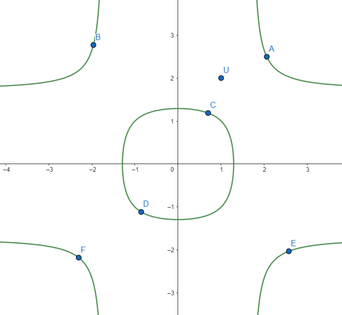
To make it easier to plot the coordinates, we use the command real to get the real part (and ignore the imaginary part).
We also print the coordinates on the form $(x_1,x_2)$ (instead of as column vectors), since that's the format that GeoGebra uses.
for i=1:length(sol)
    if is_real(certificates(cert_res)[i])
        display(i) # print out
        display((real(sol[i][2]),real(sol[i][3])))
    end
end
1
(0.6974628316032541, 1.1868540198708355)
4
(2.0594737601345003, 2.4944107570298666)
7
(-1.9641008231775792, 2.7683349808147066)
10
(2.570315873979099, -2.0270918252578882)
11
(-0.8541685916254985, -1.112741129782544)
12
(-2.3052655483869082, -2.1744935723311904)
Here's a link to what this looks like in GeoGebra: https://www.geogebra.org/m/nercedxu.
We need to make sure we haven't missed any solutions of the system!
You can try to prove this by computing the dimension of the coordinate ring in OSCAR, which would show that, indeed, there are 12 complex solutions.
Alternatively, you will see in Week 7 of the course that the mixed volume can be used to show that there are at most 12 solutions.
@var x y z t p[1:3] v[1:3]
(x, y, z, t, Variable[p₁, p₂, p₃], Variable[v₁, v₂, v₃])
f = 81*(x^3+y^3+z^3)-189*(x^2*y+x^2*z+x*y^2+x*z^2+y^2*z+y*z^2)+54*x*y*z+126*(x*y+x*z+y*z)-9*(x^2+y^2+z^2)-9*(x+y+z)+1
parametrized_line = p+t*v
3-element Vector{Expression}:
 p₁ + t*v₁
 p₂ + t*v₂
 p₃ + t*v₃
line_evaluated_at_surface = subs(f, [x;y;z] => parametrized_line)
coeffs = coefficients(line_evaluated_at_surface,[t])
4-element Vector{Expression}:
                                                                                                                                                                                                                                                                 -189*v₂*v₁^2 - 189*v₂*v₃^2 - 189*v₂^2*v₁ - 189*v₂^2*v₃ - 189*v₃*v₁^2 - 189*v₃^2*v₁ + 54*v₂*v₃*v₁ + 81*v₁^3 + 81*v₂^3 + 81*v₃^3
                                                                 243*v₁^2*p₁ - 189*v₁^2*p₂ - 189*v₁^2*p₃ + 126*v₂*v₁ + 126*v₂*v₃ - 189*v₂^2*p₁ + 243*v₂^2*p₂ - 189*v₂^2*p₃ + 126*v₃*v₁ - 189*v₃^2*p₁ - 189*v₃^2*p₂ + 243*v₃^2*p₃ - 378*v₂*v₁*p₁ - 378*v₂*v₁*p₂ + 54*v₂*v₁*p₃ + 54*v₂*v₃*p₁ - 378*v₂*v₃*p₂ - 378*v₂*v₃*p₃ - 378*v₃*v₁*p₁ + 54*v₃*v₁*p₂ - 378*v₃*v₁*p₃ - 9*v₁^2 - 9*v₂^2 - 9*v₃^2
 -9*v₁ - 9*v₂ - 9*v₃ - 18*v₁*p₁ + 243*v₁*p₁^2 + 126*v₁*p₂ - 189*v₁*p₂^2 + 126*v₁*p₃ - 189*v₁*p₃^2 + 126*v₂*p₁ - 189*v₂*p₁^2 - 18*v₂*p₂ + 243*v₂*p₂^2 + 126*v₂*p₃ - 189*v₂*p₃^2 + 126*v₃*p₁ - 189*v₃*p₁^2 + 126*v₃*p₂ - 189*v₃*p₂^2 - 18*v₃*p₃ + 243*v₃*p₃^2 - 378*v₁*p₁*p₂ - 378*v₁*p₁*p₃ + 54*v₁*p₂*p₃ - 378*v₂*p₁*p₂ + 54*v₂*p₁*p₃ - 378*v₂*p₂*p₃ + 54*v₃*p₁*p₂ - 378*v₃*p₁*p₃ - 378*v₃*p₂*p₃
                                                                                                                                                                          1 - 9*p₁ - 9*p₂ - 9*p₃ + 126*p₁*p₂ - 189*p₁*p₂^2 + 126*p₁*p₃ - 189*p₁*p₃^2 - 189*p₁^2*p₂ - 189*p₁^2*p₃ + 126*p₂*p₃ - 189*p₂*p₃^2 - 189*p₂^2*p₃ + 54*p₁*p₂*p₃ - 9*p₁^2 + 81*p₁^3 - 9*p₂^2 + 81*p₂^3 - 9*p₃^2 + 81*p₃^3
p_hyperplane = 7 + p[1] + 3*p[2] + 5*p[3]
v_hyperplane = 11 + 3*v[1] + 5*v[2] + 7*v[3]
F = System(vcat(coeffs,p_hyperplane,v_hyperplane))
System of length 6
 6 variables: p₁, p₂, p₃, v₁, v₂, v₃

 -189*v₂*v₁^2 - 189*v₂*v₃^2 - 189*v₂^2*v₁ - 189*v₂^2*v₃ - 189*v₃*v₁^2 - 189*v₃^2*v₁ + 54*v₂*v₃*v₁ + 81*v₁^3 + 81*v₂^3 + 81*v₃^3
 243*v₁^2*p₁ - 189*v₁^2*p₂ - 189*v₁^2*p₃ + 126*v₂*v₁ + 126*v₂*v₃ - 189*v₂^2*p₁ + 243*v₂^2*p₂ - 189*v₂^2*p₃ + 126*v₃*v₁ - 189*v₃^2*p₁ - 189*v₃^2*p₂ + 243*v₃^2*p₃ - 378*v₂*v₁*p₁ - 378*v₂*v₁*p₂ + 54*v₂*v₁*p₃ + 54*v₂*v₃*p₁ - 378*v₂*v₃*p₂ - 378*v₂*v₃*p₃ - 378*v₃*v₁*p₁ + 54*v₃*v₁*p₂ - 378*v₃*v₁*p₃ - 9*v₁^2 - 9*v₂^2 - 9*v₃^2
 -9*v₁ - 9*v₂ - 9*v₃ - 18*v₁*p₁ + 243*v₁*p₁^2 + 126*v₁*p₂ - 189*v₁*p₂^2 + 126*v₁*p₃ - 189*v₁*p₃^2 + 126*v₂*p₁ - 189*v₂*p₁^2 - 18*v₂*p₂ + 243*v₂*p₂^2 + 126*v₂*p₃ - 189*v₂*p₃^2 + 126*v₃*p₁ - 189*v₃*p₁^2 + 126*v₃*p₂ - 189*v₃*p₂^2 - 18*v₃*p₃ + 243*v₃*p₃^2 - 378*v₁*p₁*p₂ - 378*v₁*p₁*p₃ + 54*v₁*p₂*p₃ - 378*v₂*p₁*p₂ + 54*v₂*p₁*p₃ - 378*v₂*p₂*p₃ + 54*v₃*p₁*p₂ - 378*v₃*p₁*p₃ - 378*v₃*p₂*p₃
 1 - 9*p₁ - 9*p₂ - 9*p₃ + 126*p₁*p₂ - 189*p₁*p₂^2 + 126*p₁*p₃ - 189*p₁*p₃^2 - 189*p₁^2*p₂ - 189*p₁^2*p₃ + 126*p₂*p₃ - 189*p₂*p₃^2 - 189*p₂^2*p₃ + 54*p₁*p₂*p₃ - 9*p₁^2 + 81*p₁^3 - 9*p₂^2 + 81*p₂^3 - 9*p₃^2 + 81*p₃^3
 7 + p₁ + 3*p₂ + 5*p₃
 11 + 3*v₁ + 5*v₂ + 7*v₃
res = solve(F, start_system = :total_degree)
Tracking 81 paths... 100%|██████████████████████████████| Time: 0:00:08
  # paths tracked:                  81
  # non-singular solutions (real):  27 (27)
  # singular endpoints (real):      0 (0)
  # total solutions (real):         27 (27)
Result with 27 solutions
========================
• 81 paths tracked
• 27 non-singular solutions (27 real)
• random_seed: 0xdbc91ec8
• start_system: :total_degree
sol = solutions(res)
27-element Vector{Vector{ComplexF64}}:
 [-3.1620226591665967 + 4.71953478672989e-55im, 1.1724069756247721 - 5.6761864793649275e-55im, -1.471039653541544 + 2.462123548655205e-55im, -2.487398367265553 + 3.659132983382351e-55im, 0.8497967345311054 - 4.3021447060131874e-55im, -1.1123983672655526 + 1.5046753100646012e-55im]
 [-1.960921556706866 - 1.7663216158335846e-49im, -4.257431895591226 - 3.788643976555687e-49im, 1.5466434486961087 + 2.626408947151534e-49im, -1.24535599249993 - 6.421943645225428e-50im, -2.7847006554165614 - 1.5174204022062489e-49im, 0.9513673220832282 + 1.3591426170304767e-49im]
 [-6.690110314363694 + 1.3688783712967305e-50im, -2.960023851754312 + 6.884522478961843e-51im, 1.7140363739253262 - 6.868535483015247e-51im, -2.8959761093511047 + 2.6127319089866092e-51im, -1.236729444604445 + 1.663136976281124e-51im, 0.5530822215822199 - 2.3076739251076782e-51im]
 [0.4862314044720563 - 4.9444008924937546e-46im, -0.572824169777703 + 1.7884537781110918e-46im, -1.1535517790277894 - 8.413863307370232e-48im, 0.45767653215896664 - 1.0051305879361115e-45im, -0.5991063585226795 + 4.587747169579052e-46im, -1.3396425434090717 + 1.0299766086811285e-46im]
 [1.5 + 0.0im, -0.3333333333333333 + 0.0im, -1.5 + 0.0im, 2.75 + 0.0im, 1.3745303651574703e-31 + 0.0im, -2.75 + 0.0im]
 [-4.305413494079029e-25 - 2.4092468445198007e-39im, 4.333333333333333 - 7.210521378029779e-39im, -4.0 + 4.807731716833587e-39im, -8.816057041260357e-25 - 2.0878226079668315e-39im, 5.5 - 1.0460636984246186e-38im, -5.5 + 8.365639728142012e-39im]
 [0.7036893258332633 + 3.2359679444877937e-59im, -1.3998644896874035 - 4.6672614583958563e-60im, -0.7008191713542105 - 3.733809166716685e-60im, 0.2832655781770351 - 2.4892061111444567e-60im, -1.483197823020737 + 2.800356875037514e-60im, -0.6334010884896315 - 1.2446030555722283e-60im]
 [-0.7870226591665965 + 1.6262068678489502e-42im, 0.6498644896874036 - 1.9337918807682476e-42im, -1.6325141619791228 + 8.344732355054286e-43im, -0.7415989115103685 + 1.0296040466626593e-42im, 0.5665311563540703 - 1.5526386984718973e-42im, -1.6582655781770352 + 6.6841936748293774e-43im]
 [-0.3333333333333333 - 1.0399703995872648e-54im, 3.3333333333333335 - 3.1810859281492807e-54im, -3.3333333333333335 + 2.1207239520995205e-54im, 7.012096901446298e-31 - 1.9575913403995574e-54im, 5.5 - 9.95108931369775e-54im, -5.5 + 7.83036536159823e-54im]
 [4.0 - 2.5489470578119236e-57im, -3.6666666666666665 + 2.5489470578119236e-57im, 9.61990158054697e-31 - 6.372367644529809e-58im, 5.5 - 1.5293682346871542e-56im, -5.5 + 1.0195788231247695e-56im, 8.796994336990591e-30 - 2.5489470578119236e-57im]
 [-11.508384612916164 + 9.656538294253463e-39im, -5.2036461922219415 + 4.310797650220863e-39im, 4.023864637916398 - 4.51778624898321e-39im, -3.8669998526227993 + 1.0251563253368924e-39im, -1.7293749078892495 + 4.41027863080021e-40im, 1.3211248710449492 - 7.543722126876934e-40im]
 [-3.0417869600276117 - 5.0752594526998685e-46im, 1.0172686142221474 - 1.0508370026904561e-44im, -1.4020037765277662 + 6.406424571031866e-45im, -2.184949259431694 + 1.1820034653911726e-46im, 0.41728817670449764 - 6.484426536331197e-45im, -0.933084729318201 + 4.580904891921216e-45im]
 [-2.8333333333333335 - 1.1732497433461347e-51im, -5.275009285368947e-30 - 3.6854919635255667e-51im, -0.8333333333333334 + 2.4430739928186476e-51im, -2.0625 + 1.4616682008316695e-52im, -3.502064321621407e-30 - 2.3386691213306712e-51im, -0.6875 + 1.610445142702036e-51im]
 ⋮
 [2.6666666666666665 + 3.103035319400875e-40im, -2.6666666666666665 - 2.32996698260216e-40im, -0.3333333333333333 + 7.771040763759706e-41im, 5.5 + 1.1113529964744405e-39im, -5.5 - 9.258883421241223e-40im, -1.3505298697383722e-26 + 1.8515076349430943e-40im]
 [-3.6666666666666665 - 3.74672176898848e-43im, -1.1111111111111112 - 2.8695965114751645e-43im, -1.3476016180581918e-24 + 2.4711022606827946e-43im, -2.357142857142857 - 1.1999986556312813e-43im, -0.7857142857142857 - 1.1869435898601302e-43im, -7.065164484904217e-25 + 1.3621058979007323e-43im]
 [2.8333333333333335 + 2.419269682119389e-49im, 0.3333333333333333 + 1.1923036323926904e-49im, -2.1666666666666665 - 1.1994031636538728e-49im, 2.75 + 5.6278401926878795e-49im, -2.928251680180396e-26 + 1.87594673089596e-49im, -2.75 - 3.75189346179192e-49im]
 [-0.6 - 3.68407205727333e-48im, -2.1333333333333333 - 4.218290903703008e-48im, -2.689447706951891e-25 + 3.267788953676471e-48im, -0.6111111111111112 - 1.9975575252051547e-48im, -1.8333333333333333 - 2.0344750877633032e-48im, -1.8675177525840145e-25 + 2.309268709519657e-48im]
 [-1.6713106741667367 - 6.933135997248432e-55im, -3.672406975624772 - 1.3254524700622003e-54im, 1.1377063202082107 + 9.278167290435402e-55im, -0.9501016327344473 - 3.1606943516867853e-55im, -2.2247967345311053 - 4.639083645217701e-55im, 0.4248983672655527 + 4.6900625863739395e-55im]
 [5.333333333333333 + 0.0im, -4.666666666666667 + 0.0im, 0.3333333333333333 + 0.0im, 5.5 + 0.0im, -5.5 + 0.0im, -2.2183724849854266e-29 + 0.0im]
 [0.3333333333333333 + 0.0im, 5.333333333333333 + 0.0im, -4.666666666666667 + 0.0im, 0.0 + 0.0im, 5.5 + 0.0im, -5.5 + 0.0im]
 [-0.3333333333333333 - 4.8372822988492685e-42im, -5.49678278758001e-27 + 5.784560060732845e-42im, -1.3333333333333333 - 2.5027190572841233e-42im, -0.4583333333333333 - 3.1361059631589406e-42im, -4.5059734906224194e-27 + 4.8148615234200715e-42im, -1.375 - 2.0963425026299263e-42im]
 [2.1666666666666665 + 3.61009516871681e-43im, 1.2473468633354639e-26 + 1.8234396267026682e-43im, -1.8333333333333333 - 1.815557322840841e-43im, 2.75 + 8.835186817567972e-43im, 2.5975611887117477e-26 + 2.94097515200171e-43im, -2.75 - 5.887205173244638e-43im]
 [-0.824948720417169 + 8.712221389005598e-60im, 0.7592017477774974 - 3.002604871568001e-59im, -1.6905313045830646 + 1.6335415104385497e-59im, -0.6411968686886763 + 1.2873862856075237e-59im, 0.28675195706957735 - 2.6447814930909852e-59im, -1.5014527398974082 + 1.3379482847401455e-59im]
 [0.5673032968198342 + 8.320209631928601e-44im, -1.3908533412281439 + 7.466293380230666e-45im, -0.6789486546270804 - 2.1150848695902708e-44im, 0.528887501756168 + 1.0159413866354924e-43im, -1.5480806819778334 - 3.4244231221937717e-44im, -0.6923227279113339 - 1.9092691576425633e-44im]
 [0.6598462878896617 + 3.111507638930571e-61im, -0.6027831581722148 - 6.223015277861142e-61im, -1.1702993626746034 + 3.111507638930571e-61im, 0.2453559924999299 - 5.600713750075028e-60im, -0.5486326779167718 + 2.0613738107915032e-60im, -1.2847006554165614 + 9.334522916791713e-61im]
cert_res = certify(F,res)
CertificationResult
===================
• 27 solution candidates given
• 27 certified solution intervals (27 real, 0 complex)
• 27 distinct certified solution intervals (27 real, 0 complex)
To make it easier to copy and paste the $p$ and $v$ for each solution, we print them in the following way. We also use the real command to ignore the imaginary parts.
for i=1:length(sol)
    print(i)
    print("\n")
    print("p: ")
    print(real(sol[i][1:3]))
    print("\n")
    print("v: ")
    print(real(sol[i][4:6]))
    print("\n\n")
end
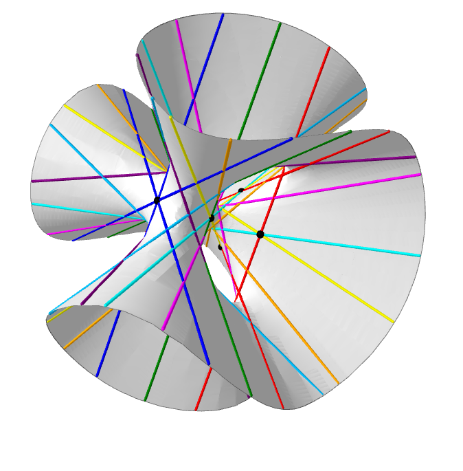
1
p: [-3.1620226591665967, 1.1724069756247721, -1.471039653541544]
v: [-2.487398367265553, 0.8497967345311054, -1.1123983672655526]

2
p: [-1.960921556706866, -4.257431895591226, 1.5466434486961087]
v: [-1.24535599249993, -2.7847006554165614, 0.9513673220832282]

3
p: [-6.690110314363694, -2.960023851754312, 1.7140363739253262]
v: [-2.8959761093511047, -1.236729444604445, 0.5530822215822199]

4
p: [0.4862314044720563, -0.572824169777703, -1.1535517790277894]
v: [0.45767653215896664, -0.5991063585226795, -1.3396425434090717]

5
p: [1.5, -0.3333333333333333, -1.5]
v: [2.75, 1.3745303651574703e-31, -2.75]

6
p: [-4.305413494079029e-25, 4.333333333333333, -4.0]
v: [-8.816057041260357e-25, 5.5, -5.5]

7
p: [0.7036893258332633, -1.3998644896874035, -0.7008191713542105]
v: [0.2832655781770351, -1.483197823020737, -0.6334010884896315]

8
p: [-0.7870226591665965, 0.6498644896874036, -1.6325141619791228]
v: [-0.7415989115103685, 0.5665311563540703, -1.6582655781770352]

9
p: [-0.3333333333333333, 3.3333333333333335, -3.3333333333333335]
v: [7.012096901446298e-31, 5.5, -5.5]

10
p: [4.0, -3.6666666666666665, 9.61990158054697e-31]
v: [5.5, -5.5, 8.796994336990591e-30]

11
p: [-11.508384612916164, -5.2036461922219415, 4.023864637916398]
v: [-3.8669998526227993, -1.7293749078892495, 1.3211248710449492]

12
p: [-3.0417869600276117, 1.0172686142221474, -1.4020037765277662]
v: [-2.184949259431694, 0.41728817670449764, -0.933084729318201]

13
p: [-2.8333333333333335, -5.275009285368947e-30, -0.8333333333333334]
v: [-2.0625, -3.502064321621407e-30, -0.6875]

14
p: [-3.8854259082307496e-30, -0.2962962962962963, -1.2222222222222223]
v: [-2.8465689853157097e-30, -0.4230769230769231, -1.2692307692307692]

15
p: [-4.947735597546186e-27, -1.619047619047619, -0.42857142857142855]
v: [-4.392377520270594e-27, -1.5, -0.5]

16
p: [2.6666666666666665, -2.6666666666666665, -0.3333333333333333]
v: [5.5, -5.5, -1.3505298697383722e-26]

17
p: [-3.6666666666666665, -1.1111111111111112, -1.3476016180581918e-24]
v: [-2.357142857142857, -0.7857142857142857, -7.065164484904217e-25]

18
p: [2.8333333333333335, 0.3333333333333333, -2.1666666666666665]
v: [2.75, -2.928251680180396e-26, -2.75]

19
p: [-0.6, -2.1333333333333333, -2.689447706951891e-25]
v: [-0.6111111111111112, -1.8333333333333333, -1.8675177525840145e-25]

20
p: [-1.6713106741667367, -3.672406975624772, 1.1377063202082107]
v: [-0.9501016327344473, -2.2247967345311053, 0.4248983672655527]

21
p: [5.333333333333333, -4.666666666666667, 0.3333333333333333]
v: [5.5, -5.5, -2.2183724849854266e-29]

22
p: [0.3333333333333333, 5.333333333333333, -4.666666666666667]
v: [0.0, 5.5, -5.5]

23
p: [-0.3333333333333333, -5.49678278758001e-27, -1.3333333333333333]
v: [-0.4583333333333333, -4.5059734906224194e-27, -1.375]

24
p: [2.1666666666666665, 1.2473468633354639e-26, -1.8333333333333333]
v: [2.75, 2.5975611887117477e-26, -2.75]

25
p: [-0.824948720417169, 0.7592017477774974, -1.6905313045830646]
v: [-0.6411968686886763, 0.28675195706957735, -1.5014527398974082]

26
p: [0.5673032968198342, -1.3908533412281439, -0.6789486546270804]
v: [0.528887501756168, -1.5480806819778334, -0.6923227279113339]

27
p: [0.6598462878896617, -0.6027831581722148, -1.1702993626746034]
v: [0.2453559924999299, -0.5486326779167718, -1.2847006554165614]
Here's an example of some lines plotted together with the surface: https://www.math3d.org/AG5b1iNKf
Here's another very nice animation of all 27 lines: https://analyticphysics.com/Higher%20Dimensions/27%20Lines%20on%20a%20Cubic%20Surface.htm
We all know that $\mathbb{V}(x^2-5x+6)=\{2,3\}$ and $\mathbb{V}(-x^2+2x)=\{0,2\}.$
However, if we solve these univariate equations using a straight line homotopy from the total degree system, and force HomotopyContinuation.jl to pick the specific value $\gamma=1$ for the $\gamma$-trick, then something goes wrong!
Exercise: Explain in simple terms what happens, and suggest better values of $\gamma\in\mathbb{C}\setminus\{0\}$ (trial and error is fine).
Hint: Use the GeoGebra applet from the lecture (https://www.geogebra.org/m/vftzrnnx) to visualize the homotopies.
@var x
F = System([x^2-5*x+6])
solve(F, start_system = :total_degree, gamma=1)
Result with 0 solutions
=======================
• 2 paths tracked
• 0 non-singular solutions (0 real)
• random_seed: 0xf277edce
• start_system: :total_degree
@var x
F = System([-x^2+2*x])
res = solve(F, start_system = :total_degree, gamma = 1)
Result with 1 solution
======================
• 2 paths tracked
• 1 non-singular solution (1 real)
• random_seed: 0x6652e3a1
• start_system: :total_degree
Explanation: In both cases, the root count drops along the homotopy. In the first case, two paths collide in a point where the Jacobian becomes singular, and in the second case, one path goes off to infinity.
Here are better gammas:
@var x
F = System([x^2-5*x+6])
res = solve(F, start_system = :total_degree, gamma=im)
Result with 2 solutions
=======================
• 2 paths tracked
• 2 non-singular solutions (2 real)
• random_seed: 0xc352cc52
• start_system: :total_degree
@var x
F = System([-x^2+2*x])
solve(F, start_system = :total_degree, gamma = -1)
Result with 2 solutions
=======================
• 2 paths tracked
• 2 non-singular solutions (2 real)
• random_seed: 0x4efdb5dc
• start_system: :total_degree
You can choose a random complex number by wrting randn(ComplexF64) or exp(2*pi*im*rand()) (if you want to restrict to the unit circle). This is what HomotopyContinuation.jl does as default if you don't provide it with any speicific $\gamma$.
solve(F, start_system = :total_degree, gamma = randn(ComplexF64))
Result with 2 solutions
=======================
• 2 paths tracked
• 2 non-singular solutions (2 real)
• random_seed: 0x37035a07
• start_system: :total_degree
solve(F, start_system = :total_degree)
Result with 2 solutions
=======================
• 2 paths tracked
• 2 non-singular solutions (2 real)
• random_seed: 0xe8db8f9d
• start_system: :total_degree
Here we want to find a $\gamma$ for which we run into trouble when we solve the system
$$\begin{cases}x^2-y^2-1=0\\2x^2+y^2-8=0\end{cases}$$with a straight-line homotopy from the total degree system with the $\gamma$-trick.
Specifically, we'll try to cook up a $\gamma$ such that at least one of the paths run into a singular Jacobian at $t=1/2$.
This corresponds to making sure that there is a solution to the system
$$\begin{cases}H(\tfrac{1}{2},x)=0\\ \det\left(\frac{\partial H}{\partial x}\Big(\tfrac{1}{2},x\Big)\right)=0\,,\end{cases}$$which takes the following form:
$$\begin{cases}\tfrac{1}{2}\gamma(x^2-1) + \tfrac{1}{2}(-1 + x^2 - y^2)=0\\ \tfrac{1}{2}\gamma (y^2-1) + \tfrac{1}{2}(-8 + 2x^2 + y^2)=0\\ (x + \gamma x)*(y + \gamma y)+2xy=0\,.\end{cases}$$From this we can use elimination and extension in OSCAR to show that this system has solutions if and only if
which gives $\gamma\in\Big\{-6, -1, -\frac{3}{2} \pm \frac{3\sqrt{3}}{2}i\Big\}$.
Let's try one of these gammas, and see what happens!
F = System([x^2-y^2-1, 2*x^2+y^2-8])
solve(F, start_system = :total_degree, gamma=-6)
Tracking 4 paths... 100%|███████████████████████████████| Time: 0:00:04
  # paths tracked:                  4
  # non-singular solutions (real):  0 (0)
  # singular endpoints (real):      0 (0)
  # total solutions (real):         0 (0)
Result with 0 solutions
=======================
• 4 paths tracked
• 0 non-singular solutions (0 real)
• random_seed: 0x933cd3c0
• start_system: :total_degree
If we don't want to use elimination to find the gammas, we could also try to solve the system with homotopy continuation!
using LinearAlgebra #for computing determinants

@var x y gamma

homotopy = 0.5*[x^2-y^2-1, 2*x^2+y^2-8]+0.5*gamma*[x^2-1,y^2-1]

jac = [differentiate(homotopy[1],x);differentiate(homotopy[1],y);;
        differentiate(homotopy[2],x);differentiate(homotopy[2],y)]
detjac = det(jac)

S = System(vcat(homotopy,detjac))
System of length 3
 3 variables: gamma, x, y

 0.5*(-1 + x^2)*gamma + 0.5*(-1 + x^2 - y^2)
 0.5*(-1 + y^2)*gamma + 0.5*(-8 + 2*x^2 + y^2)
 2.0*x*y + (1.0*x + 1.0*x*gamma)*(1.0*y + 1.0*y*gamma)
res = solve(S, start_system = :total_degree)
Tracking 36 paths... 100%|██████████████████████████████| Time: 0:00:04
  # paths tracked:                  36
  # non-singular solutions (real):  8 (4)
  # singular endpoints (real):      0 (0)
  # total solutions (real):         8 (4)
Result with 8 solutions
=======================
• 36 paths tracked
• 8 non-singular solutions (4 real)
• random_seed: 0xa07117cf
• start_system: :total_degree
sol = solutions(res)
8-element Vector{Vector{ComplexF64}}:
 [-6.0 + 0.0im, 1.0 + 0.0im, 0.0 + 0.0im]
 [-1.5 - 2.598076211353316im, 0.0 - 8.228460455756013e-38im, 1.2541433951236578 + 1.0357971111816713im]
 [-6.0 + 0.0im, -1.0 + 0.0im, 0.0 + 0.0im]
 [-1.5 + 2.598076211353316im, 5.109273657352392e-48 - 2.1895288505075267e-47im, -1.2541433951236578 + 1.0357971111816713im]
 [-1.0 + 0.0im, -1.8708286933869707 + 0.0im, -1.1479437019748901e-41 + 0.0im]
 [-1.5 - 2.598076211353316im, -1.1210387714598537e-44 + 1.6815581571897805e-44im, -1.2541433951236578 - 1.0357971111816713im]
 [-1.0 + 0.0im, 1.8708286933869707 + 0.0im, 0.0 + 0.0im]
 [-1.5 + 2.598076211353316im, 5.739718509874451e-42 - 4.304788882405838e-42im, 1.2541433951236578 - 1.0357971111816713im]
for s in sol
    display(s[1]) #the first coordinate corresponds to the lambda
end
-6.0 + 0.0im
-1.5 - 2.598076211353316im
-6.0 + 0.0im
-1.5 + 2.598076211353316im
-1.0 + 0.0im
-1.5 - 2.598076211353316im
-1.0 + 0.0im
-1.5 + 2.598076211353316im
In this exercise, we try to solve the overdetermined system $$\begin{cases}xz - y^2=0\\y - z^2=0\\x - yz=0\\x + y + z + 1=0\,.\end{cases}$$
As explained in the slides, the trick here is to turn it into a square system by computing 3 random linear combinations of these four equations. We then solve it, and check which solutions actually correspond to solutions of the original system.
The easy solution is to just feed this to the solve command as usual.
Then HomotopyContinuation.jl will take care of the randomization and checking for you!
@var x y z
original_polynomials = [x*z - y^2, y - z^2, x - y*z, x + y + z + 1]
F = System(original_polynomials)
res = solve(F, start_system = :total_degree)
Tracking 8 paths... 100%|███████████████████████████████| Time: 0:00:08
  # paths tracked:                  8
  # non-singular solutions (real):  3 (1)
  # singular endpoints (real):      0 (0)
  # total solutions (real):         3 (1)
Result with 3 solutions
=======================
• 8 paths tracked
• 3 non-singular solutions (1 real)
• 2 excess solutions
• random_seed: 0x46a056ed
• start_system: :total_degree
Note: Certification won't work for nonsquare systems.
#certify(F,solutions(res))
Alternatively, we can do the work ourselves! We begin by picking a random matrix $A\in\mathbb{C}^{3\times 4}$ that we use to obtian the square system.
A = rand(ComplexF64,3,4)
new_polynomials = A*original_polynomials
F_new = System(new_polynomials)
res = solve(F_new, start_system = :total_degree)
Tracking 8 paths... 100%|███████████████████████████████| Time: 0:00:04
  # paths tracked:                  8
  # non-singular solutions (real):  5 (1)
  # singular endpoints (real):      0 (0)
  # total solutions (real):         5 (1)
Result with 5 solutions
=======================
• 8 paths tracked
• 5 non-singular solutions (1 real)
• random_seed: 0xc3c00807
• start_system: :total_degree
We then evaluate the original polynomials on all the solutions we found, and check if we get something that's almost equal to 0.
for s in solutions(res)
    display(F(s))
end
4-element Vector{ComplexF64}:
                     0.0 + 2.2600554338864107e-16im
                     0.0 - 1.2204619091670405e-16im
  -3.688408887122106e-17 + 0.0im
 -2.8113197155040956e-17 + 0.0im
4-element Vector{ComplexF64}:
   0.2860429780180407 + 0.13406437823812173im
 -0.17612776632945384 + 0.014258482815629359im
  -0.5624106216026782 + 0.07596012831640059im
 0.014947493312791327 - 0.03055155415656037im
4-element Vector{ComplexF64}:
 0.0 + 0.0im
 0.0 + 2.4492935982947064e-16im
 0.0 + 0.0im
 0.0 + 0.0im
4-element Vector{ComplexF64}:
 -1.1102230246251565e-16 - 2.296231923522978e-16im
                     0.0 + 1.148115961761489e-16im
  -6.933347799794049e-32 - 1.1102230246251565e-16im
 -1.1479625607879665e-17 - 1.1102230246251565e-16im
4-element Vector{ComplexF64}:
 -10233.235609938238 + 7618.888495502251im
  2856.0431985013165 - 6539.932898576095im
   8037.033169072563 - 21464.402314408133im
   801.7545608720575 + 1115.3492117827082im
Conclusion: Only three of the solutions make sense as solutions of the original system!